6. Source
To introduce a source into a GATE simulation, the user has to define the type of source (voxelized, linacBeam, phaseSpace, PencilBeam, TPSPencilBeam or GPS) and its feature (angle, energy, and position). Many activity distributions are available in GATE. At each new event, the source manager decides randomly which source decays, and generates for it one or more primary particles.
6.1. Creating a source
Different type of sources can be defined in the same GATE simulation. Each source is independent. The command to create a source is given below:
/gate/source/NAME
where “NAME” defines the name of the source.
6.1.1. Adding a source
The next step is to add the source. For this, user has to type the following GATE command:
/gate/source/addSource NAME
or:
/gate/source/addSource NAME gps
In this example, a source “NAME” is added. Once a source has been added, a series of properties must be assigned to it. These properties are: activity, type of particle(s), energy distribution, energy value or bounds, angular emission, spatial distribution and location, and half-life. The commands required to assign these properties are described in the following paragraphs.
6.1.2. Defining the type of source
Ion source
The ion source type can simulate any ion by defining its atomic number (Z), atomic weight (A), ionic charge in units of energy (Q), and its excitation energy in keV (E). It incorporates both the radioactive decay and the atomic de-excitation. This is the most “realistic” way of simulating a radionuclide; however, it is also the slowest.
To use the ion source:
/gate/source/NAME/gps/particle ion
/gate/source/NAME/gps/ion 8 15 0 0
/gate/source/NAME/setForcedUnstableFlag true
/gate/source/NAME/useDefaultHalfLife
In the above example, an ion source of oxygen-15 has been defined with Z=8, A=15, Q=0, E=0 . If it is too slow, other options are available, as described below.
Simple particles
You can choose from a long list of simple particles \(( e^{-} , e^{+}\) , gamma, etc) to use in your simulations (use the help command to obtain the full list). For example:
/gate/source/NAME/gps/particle gamma
defines a photon source and:
/gate/source/NAME/gps/particle e+
defines a positron source. If you choose to use a particle, you will have to define more properties. As an example, the correct use of a positron source simulating fluorine-18 is:
/gate/source/NAME/gps/particle e+
/gate/source/NAME/gps/energytype Fluor18
/gate/source/NAME/setForcedUnstableFlag true
/gate/source/NAME/setForcedHalfLife 6586 s
In the above example, more properties of fluorine-18 have been added by using the helper keyword Fluor18 (see below): half-life and energy distribution. Note that the branching ratios are not respected with this kind of simulation because no decay is simulated, i.e. emission is 100% positron. You may want to lower the activity by an appropriate factor to take this better point into account.
Helper keywords
These keywords are defined to help you to define the particle properties. The first three keywords define an positron energy distribution resulting from common beta emitters, and the last one defines a special two-particle source.
For instance, Fluor18 defines the positron energy spectrum of fluorine-18. Note that this keyword define only the energy spectrum, you still have to specify the particle \(e^{+}\) and the half-life.
Back-to-back This keyword is implemented for PET simulations where two annihilation photons are generated at 180 degrees. This type of source is faster to simulate than the ion source or the positron source and allows for selecting emission angle. To use the back-to-back source type:
/gate/source/NAME/setType backtoback
Note that there are no radioactive decays simulated when using the back-to-back type and that you still have to define the particle (gamma), energy type (Mono) and energy-value (0.511 MeV). The back-to-back source does not consider photon accolinearity by default, but it can be enabled with the command “setAccolinearityFlag”. If the accolinearity flag is set to True, a default value of 0.5 degrees (FWHM) is used for creating the accolinear angular distribution. However, the user can specify a custom value for accolinearity. In that case, the command “setAccoValue” expects the FWHM of the distribution:
/gate/source/NAME/setType backtoback
/gate/source/NAME/setAccolinearityFlag True
/gate/source/NAME/setAccoValue 0.5 deg
Please note, the default value of 0.5 degrees would override /gate/source/NAME/setAccoValue 0.0 deg. In case accolinearity should not be simulated, please set the “AccolinearityFlag” to False or omit the commands related to accolinearity.
Note: In the past, there has been an issue with the accolinearity flag, see https://github.com/OpenGATE/Gate/issues/381 for details.
To debug, you can save the angle of the photons in an output file with that command:
/gate/source/setDebugPositronAnnihilationFlag True
/gate/output/debugPositronAnnihilation/setFileName output/dataAcoBTB.bin
FastI124
FastI124 is a special source implementing a simplified decay scheme of the non-pure beta emitter iodine-124 in which positrons are emitted but not neutrinos, there is no nuclear recoil, gammas are emitted if their emission probability is > 1%; and no atomic de-excitation occurs (no x-rays, Auger electrons). These simplifications allow for an increase in speed with respect to the ion source while retaining important features of iodine-124, i.e. gammas may be emitted concurrently with positrons to possibly create “dirty” coincidences. Since decay is simulated, branching ratios are respected hence no activity compensation is necessary.
To use the fastI124 source:
/gate/source/NAME/setType fastI124
The source takes care of particle definitions (gamma, positron) and energy distribution so that there is no need to specify a particle or mention its energy.
Defining the activity
To define the activity of the given source, the user defines the amount of activity and its unit using the following command:
/gate/source/NAME/setActivity 5. Bq
In this example, the total activity of the source referred to as “NAME” is set to 5 Bq. The activity can be defined in Curie (Ci) as well as in Bq (Bq).
6.1.3. Defining the energy
Energy distribution
If the source does not take care of the type of energy distribution (e.g. fastI124), then it has to be explicitly defined. This can be achieved either by using a pre-defined spectrum (see helper keywords above) or by using built-in distributions.
Candidates for built-in energy distributions are: mono-energetic “Mono”, linear “Lin”, powerlaw “Pow”, exponential “Exp”, Gaussian “Gauss”, bremstrahlung “Brem”, black-body “Bbody”, cosmic diffuse gamma ray “Cdg”, user-defined histogram “UserSpectrum”, arbitrary point-wise spectrum “Arb”, and user-defined energy per nucleon histogram “Epn”. Capitalization is important: only strings given exactly as above will be recognized.
In the following example, all particles have the same energy:
/gate/source/NAME/gps/energytype Mono
Energy value
You may have to specify the energy value (or bounds) depending on the type of energy distribution you have selected. For example, for monoenergetic distributions (like back-to-back sources), you specify the energy value with:
/gate/source/NAME/gps/monoenergy 511. keV
In the case of ions, the kinetic energy must be 0 since the ions are at rest:
/gate/source/NAME/gps/monoenergy 0. ev
Any type of energy unit within the International System of Units (SI) can be used: eV, GeV, MeV, keV…
Examples
ion source for fluorine-18:
/gate/source/NAME/gps/particle ion
/gate/source/NAME/gps/ion 9 18 0 0
/gate/source/NAME/gps/monoenergy 0. keV
/gate/source/NAME/setForcedUnstableFlag true # WARNING - DEBUG - New command line to debug the use of ion particle type
/gate/source/F18/useDefaultHalfLife
positron source for flourine-18:
/gate/source/NAME/gps/particle e+
/gate/source/NAME/gps/energytype Fluor18
/gate/source/NAME/setForcedUnstableFlag true
/gate/source/NAME/setForcedHalfLife 6586 s
backtoback for fluorine-18:
/gate/source/NAME/setType backtoback
/gate/source/NAME/gps/particle gamma
/gate/source/NAME/gps/monoenergy 511. keV
/gate/source/NAME/setForcedUnstableFlag true
/gate/source/NAME/setForcedHalfLife 6586 s
fast iodine-124 source:
/gate/source/NAME/setType fastI124
/gate/source/NAME/setForcedUnstableFlag true
/gate/source/NAME/setForcedHalfLife 360806 s
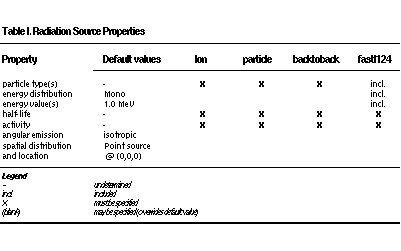
Fig. 6.1 Properties of radioactive source
Another way to define the energy of a radioactive source is to use the energytype UserSpectrum. You can define 3 different user spectra: a discrete spectrum, a histogram or a linear interpolated spectrum
Example:
 ###################### Mode 1: Discrete Spectrum ###################
/gate/source/addsource spectrumLine gps
/gate/source/spectrumLine/gps/particle gamma
/gate/source/spectrumLine/gps/energytype UserSpectrum
/gate/source/spectrumLine/gps/setSpectrumFile ../data/DiscreteSpectrum.txt
/gate/source/spectrumLine/setIntensity 1
 #################### Mode 1: Discrete Spectrum ####################


 #################### Mode 2: Histogram ####################
/gate/source/addSource histogram gps
/gate/source/histogram/gps/particle e-
/gate/source/histogram/gps/energytype UserSpectrum
/gate/source/histogram/gps/setSpectrumFile ../data/Histogram.txt
/gate/source/histogram/setIntensity 10
#################### Mode 2: Histogram ####################


#################### Mode 3: Linear interpolation spectrum ####################
/gate/source/addSource interpolationSpectrum gps
/gate/source/interpolationSpectrum/gps/particle e-
/gate/source/interpolationSpectrum/gps/energytype UserSpectrum
/gate/source/interpolationSpectrum/gps/setSpectrumFile ../data/InterpolationSpectrum.txt
/gate/source/interpolationSpectrum/setIntensity 10
#################### Mode 3: Linear interpolation spectrum ####################
The user spectra are specified by a text file. The first number on the first line indicates the mode as follows: 1 - discrete, 2 - histogram, and 3 - interpolated spectrum. The second number on the first line specifies the energy, in MeV, of the lower edge of the first bin in histogram mode. (Though ignored in the discrete and interpolated modes, it must be present for the file to parse correctly.) The remaining lines specify the energy, in MeV, and the associated probability weighting. The probabilities will normalized by the GATE software.
The discrete spectrum generates particles with one of the listed energies:
################DiscreteSpectrum.txt ###################
1   0
0.2   0.2
0.4   0.4
0.6   0.6
0.8   0.8
1.0   1.0
1.2   0.8
1.4   0.6
1.6   0.4
1.8   0.2
###################################################
In histogram mode, the energy specified on each line corresponds to the upper edge of the respective bin. The energies of the generated particles will be between the minimum energy, specified on the first line of the file, and the upper edge of the last bin. Within each bin, the energies are distributed uniformly:
################## Histogram.txt #####################
2   2
2.2   0.2
2.4   0.4
2.6   0.6
2.8   0.8
3.0   1
3.2   0.8
3.4   0.6
3.6   0.4
3.8   0.2
##################################################
In interpolated mode, the energy of the generated particle will fall between the first and last energy specified, according to the probability distribution created by piecewise-linear interpolation between the points provided:
################ InterpolationSpectrum.txt #############
3   0
4.2   0.2
4.4   0.4
4.6   0.6
4.8   0.8
5.0   1
5.2   0.8
5.4   0.6
5.6   0.4
5.8   0.2
#################################################
The following image present the result obtain for the 3 examples (available in example_UserSpectrum repository)
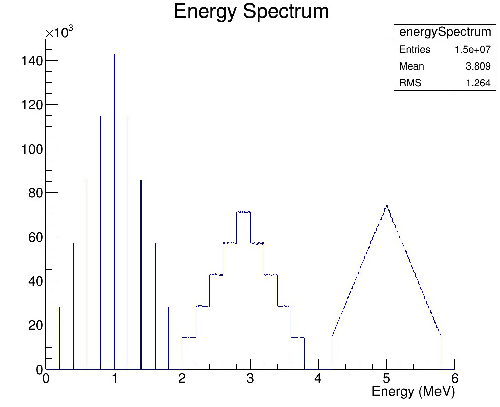
Fig. 6.2 3 different User spectra
6.1.4. Defining the angular distribution of the emission
An emission angle distribution can be defined with the angular span using:
/gate/source/NAME/gps/angtype iso
/gate/source/NAME/gps/mintheta 90. deg
/gate/source/NAME/gps/maxtheta 90. deg
/gate/source/NAME/gps/minphi 0. deg
/gate/source/NAME/gps/maxphi 360. deg
In this case, all particles have the same polar angle (theta) of 90 degrees. They are all emitted along directions orthogonal to the z-axis. The particles are emitted with an azimuthal angle (phi) between 0 and 360 degrees, along all possible directions.
By default, a full span of 0-180 degrees for the polar angle and 0-360 degrees for the azimuthal angle are defined. The emission span can be reduced for back-to-back sources to speed up the simulation.
6.1.5. Defining the shape of the source
The last step is to define its geometry. The following command defines the type of source distribution:
/gate/source/NAME/gps/type Volume
In the above description, a volumic source distribution has been chosen. Other types of source distribution can be used: Point, Beam, Plane, or Surface. The default value is Point.
For a Plane source, the source shape type can be Circle, Annulus, Ellipsoid, Square, or Rectangle. For both Surface and Volume sources, this can be Sphere, Ellipsoid, Cylinder, or Para. The default source is a Point source and so Shape is not set to any of the above types. Each shape has its own parameters:
/gate/source/NAME/gps/shape Cylinder
/gate/source/NAME/gps/radius 1. cm
/gate/source/NAME/gps/halfz 1. mm
In the previous commands, the source is a cylinder with a radius of 1 cm and a length of 2 mm. Very often, the half-length is given rather than the full length.
To define a circle, the radius (radius) should be set. (In reality it is not really a circle but a disk).
To define an annulus, the inner (radius0) and outer radii (radius) should be given.
To define an ellipse, square , or rectangle, the half-lengths along x (halfx) and y (halfy) have to be given.
To define a sphere, only the radius (radius) only has to be specified.
To define an ellipsoid, its half-lenghths in x (halfx), y (halfy), and z (halfz) have to be given.
To define a cylinder with its axis along the z-axis, only the radius (radius) and the z half-length (halfz) have to be specified.
To define parallelepipeds, the x (halfx), y (halfy), and z (halfz) half-lengths, and the angles alpha (paralp), theta (parthe), and phi (parphi) have to be given.
6.1.6. Define the placement of the source
The position of the source distribution can be defined using:
/gate/source/NAME/gps/centre 1. 0. 0. cm
In that example, the centre of the source distribution is 1 cm off-centered along the x-axis.
6.1.7. Movement of a source
6.1.7.1. Attach to a volume
The source can be attached to a volume:
/gate/source/[Source name]/attachTo [Volume Name]
If the volume moves during the simulation, the source moves along with the volume. Note that when attaching a source to a volume, the source’s placement becomes relative to the volume.
6.1.7.2. Confining a source
Note: this is the old way of moving a source. It is very inefficient. Please consider using the “Attach to a volume” method instead.
To define sources in movement, the source distribution have to be confined in a Geant4 volume. This volume will be animated using the usual GATE command as described in Chapter 4 of this manual.
The command:
/gate/source/NAME/gps/confine NAME_phys
specifies that the emission must be confined to a volume of the Geant4 geometry. In this case, the emission distribution is the intersection of the General Particle Source (GPS) and the Geant4 volume. The Geant4 volume must be specified by its physical volume name: GATEname + ‘_phys’.
One should note that the confinment slows down the simulation, the confinement volume must have an intersection with the GPS shape, and the confinement volume must not be too large as compared to the GPS shape.
A complete example of a moving source can be found in the SPECT benchmark or in the macro hereafter:
# Define the shape/dimensions of the moving source
/gate/MovingSource/geometry/setRmax 5. cm
/gate/MovingSource/geometry/setRmin 0. cm
/gate/MovingSource/geometry/setHeight 20. cm
/gate/MovingSource/moves/insert translation
/gate/MovingSource/translation/setSpeed 0 0 0.04 cm/s


# Define the shape/dimensions of the large sourcecontainer
# that should contain the full trajectory of the moving source
/gate/source/SourceContainer/gps/type Volume
/gate/source/SourceContainer/gps/shape Cylinder
/gate/source/SourceContainer/gps/radius 4. cm
/gate/source/SourceContainer/gps/halfz 30. cm
# Define the placement of the SourceContainer
/gate/source/SourceContainer/gps/centre 0. 0. 0. cm
# Define the source as a gamma source
/gate/source/SourceContainer/gps/particle gamma
# Define the gamma energy
/gate/source/SourceContainer/gps/energy 140. keV
# Set the activity of the source
/gate/source/SourceContainer/setActivity 5000. Bq
# Define a confinement and confine the large container to
# the MovingSource at a position defined by the time and
# the translation speed
/gate/source/SourceContainer/gps/confine MovingSource_phys
6.1.7.3. Example: two gammas
The following example gives a script to insert a point source of back-to-back type:
# A new source with an arbitrary name #(``twogamma'') is created
/gate/source/addSource twogamma
# The total activity of the source is set
/gate/source/twogamma/setActivity 0.0000001 Ci
# The source emits pairs of particles back-to-back
/gate/source/twogamma/setType backtoback
# The particles emitted by the source are gammas
/gate/source/twogamma/gps/particle gamma
# The gammas have an energy of 511 keV
/gate/source/twogamma/gps/energytype Mono
/gate/source/twogamma/gps/monoenergy 0.511 MeV
# The source is a full sphere with radius 0.1 mm,
# located at the centre of the FOV
/gate/source/twogamma/gps/type Volume
/gate/source/twogamma/gps/shape Sphere
/gate/source/twogamma/gps/radius 0.1 mm
/gate/source/twogamma/gps/centre 0. 0. 0. cm
# The angular distribution of emission angles is isotropic
/gate/source/twogamma/gps/angtype iso
# The parameters below mean that the source emits
# at all angles along the z axis
/gate/source/twogamma/gps/mintheta 0. deg
/gate/source/twogamma/gps/maxtheta 180. deg
# Uncomment the parameters below if you want the source
# to emit in an XY (transverse) plane
/gate/source/twogamma/gps/mintheta 90. deg
/gate/source/twogamma/gps/maxtheta 90. deg
# The parameters below mean that the source emits
# at all angles in the transverse (XY) directions
/gate/source/twogamma/gps/minphi 0. deg
/gate/source/twogamma/gps/maxphi 360. deg
6.1.8. Defining a cold source
To define a cold (i.e. with no activity) volume in a phantom, a dedicated command is available.
The command:
/gate/source/NAME/gps/Forbid Volume_Name
The following example explains how to use this option. First you must define a volume that defines the cold region:
/gate/world/daughters/name cold_area
/gate/world/daughters/insert cylinder
/gate/cold_area/vis/forceWireframe
/gate/cold_area/vis/setColor green
/gate/cold_area/geometry/setRmax 3.0 cm
/gate/cold_area/geometry/setHeight 1. cm
Then you describe your source with the Forbid command:
/gate/source/addSource number1
/gate/source/number1/setActivity 100000. Bq
/gate/source/number1/gps/particle gamma
/gate/source/number1/setType backtoback
/gate/source/number1/gps/type Volume
/gate/source/number1/gps/shape Cylinder
/gate/source/number1/gps/radius 5. cm
/gate/source/number1/gps/halfz 0.5 cm
/gate/source/number1/gps/centre 0. 0. 0. cm
/gate/source/number1/gps/monoenergy 511. keV
/gate/source/number1/gps/angtype iso
/gate/source/number1/gps/Forbid cold_area_phys
/gate/source/number1/dump 1
/gate/source/list
It is important to remember that the /gate/run/initialize command must have been executed prior to using the Forbid command because phantom geometries are not available until after they are initialized.
6.1.9. Visualizing a source
To check that sources are at the right location in the geometry, you can use the following command:
/gate/source/[Source name]/visualize
along with a real time viewer (e.g. OpenGL). To visualize a source, Gate will randomly pick a certain number of points within the source and display them on the screen, along with the geometry. The full syntax is:
/gate/source/[Source name]/visualize count color size
where name is the name of the source, count is the number of random points to pick up (must be > 0 and <= 10000), color is the color to assign to those points (valid colors are: white, gray, grey, black, red, green, blue, cyan, magenta, yellow), and size is the screen size (in pixels) of each point (must be > 0 and <= 20 ).
Depending on the size and shape of the source, more or fewer points may be necessary.
Example:
/gate/source/backgroundSource/visualize 2000 yellow 3
/gate/source/hotRegion/visualize 5000 red 2
6.1.10. Intensity
If several sources have been added and no activity is defined, user can use intensity to define the source priorities. A high intensity correspond to a high priority. For each event, the source is randomly selected taking into account the intensity of each sources:
/gate/source/MyBeam/setIntensity [value]
6.2. Pencil Beam source
Warning
Prior to GATE 9.2, the time column did not produce usable output due to an uninitialized variable in the pencil beam source.
This also affects the simulation of neutrons, which may be partially or entirely cut from all events of the run.
If you rely on the global event time or the simulation of neutrons, make sure to use GATE 9.2 or newer.
The simulation source can be a pencil beam. This source allows for characterizing a beam of particles having energy and optical properties. This beam can be used for instance in order to characterize a clinical beam interacting in a passive beam line or to characterize a spot from an active scanning beam delivery system.
Create the source:
/gate/source/addSource [Source name] PencilBeam
One can select the type of particle used for the pencil beam (proton, e-, etc.):
/gate/source/ [Source name] /setParticleType [particle_type]
Alternatively, one can define a specific type of ion, by defining the particle type as “GenericIon” and then specifying the particle parameters of the ion to be generated: Z: AtomicNumber, A: AtomicMass, Q: Charge of Ion (in unit of e), E: Excitation energy (in keV). As an example, the definition of a C12 ion beam is given:
/gate/source/  [Source name]  /setParticleType GenericIon
/gate/source/PBS/setIonProperties 6 12 6 0
The energy spectrum of the source is Gaussian and is defined by a mean energy and standard deviation:
/gate/source/ [Source name] /setEnergy [mean_energy] [Unit]
/gate/source/ [Source name] /setSigmaEnergy [energy_standard_deviation] [Unit]
The source position can be set as follows:
/gate/source/ [Source name] /setPosition [Pos_X Pos_Y Pos_Z] [Unit]
The pencil beam shape is Gaussian. The spot size can is defined by the standard deviation of the normal probability density function in x and y directions. The beam default direction being +z:
/gate/source/ [Source name] /setSigmaX [spot_size_X] [Unit]
/gate/source/ [Source name] /setSigmaY [spot_size_Y] [Unit]
The beam is also characterized by its divergences: Theta in the XoZ plan and Phi in the YoZ plan. The beam divergence is defined by the standard deviation of the normal probability density function:
/gate/source/ [Source name] /setSigmaTheta [divergence_Theta] [Unit]
/gate/source/ [Source name] /setSigmaPhi [divergence_Phi] [Unit]
The correlation between spot size and divergence (in the two plans) is characterized by the beam emittance. The beam emittance is defined by the standard deviation of the normal probability density function. The Emittance of the beam has to be lower (or equal) than the ellipse phase space area: [Emittance_X_Theta] <= Pi* [divergence_Theta] * [spot_size_X] and [Emittance_Y_Phi] <= Pi* [divergence_Phi] * [spot_size_Y].
Please note that for emittance, the unit cannot be selected and has to be “mm*mrad”:
/gate/source/ [Source name] /setEllipseXThetaEmittance [Emittance_X_Theta] mm*mrad
/gate/source/ [Source name] /setEllipseYPhiEmittance [Emittance_Y_Phi] mm*mrad
When defining the beam parameters, one can define the beam convergence or divergence in the two plans (XoZ and YoZ), by setting the “RotationNorm” either to “positive” for a convergent beam or to “negative” for a divergent beam:
/gate/source/ [Source name] /setEllipseXThetaRotationNorm [negative or positive]
/gate/source/ [Source name] /setEllipseYPhiRotationNorm [negative or positive]
Users can also define the direction of the beam, which is by default +z (0 0 1), by rotating the beam along the x, y and z axis. For instance, to rotate the beam direction around the x-axis by 90°:
/gate/source/ [Source name] /setRotationAxis 1 0 0
/gate/source/ [Source name] /setRotationAngle 90 deg
A TestFlag can be turned on for advanced testing of the source only. It provides additional output:
/gate/source/ [Source name] /setTestFlag true
The number of particles simulated is defined using the conventional command:
/gate/application/setTotalNumberOfPrimaries [number_of_primaries]
Example
In the following example, we defined a 180 MeV proton beam, with 1 MeV energy spread. The beam is asymmetrical and convergent. The direction is -Y:
/gate/source/addSource PBS PencilBeam
/gate/source/PBS/setParticleType proton
/gate/source/PBS/setEnergy 188.0 MeV
/gate/source/PBS/setSigmaEnergy 1.0 MeV
/gate/source/PBS/setPosition 0 0 0 mm
/gate/source/PBS/setSigmaX 2 mm
/gate/source/PBS/setSigmaY 4 mm
/gate/source/PBS/setSigmaTheta 3.3 mrad
/gate/source/PBS/setSigmaPhi 3.8 mrad
/gate/source/PBS/setEllipseXThetaEmittance 15 mm*mrad
/gate/source/PBS/setEllipseXThetaRotationNorm negative
/gate/source/PBS/setEllipseYPhiEmittance 20 mm*mrad
/gate/source/PBS/setEllipseYPhiRotationNorm negative
/gate/source/PBS/setRotationAxis 1 0 0
/gate/source/PBS/setRotationAngle 90 deg
/gate/application/setTotalNumberOfPrimaries 10
Pencil beam source coordinate system
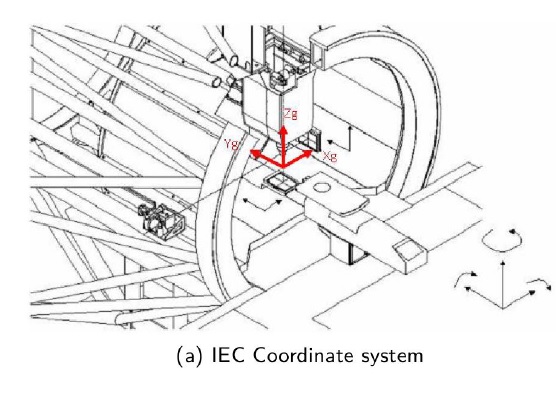
Fig. 6.3 PBS coordinate
6.3. TPS Pencil Beam source
The source of the simulation can be a stack of pencil beams. This source has been designed in order to allow the simulation of real treatment plans for active beam scanning delivery techniques.
For a more practical understanding of the source, the user is invited to execute the TPS source validation procedure available in the GitHub GateContrib of Gate, in the GATE-RTion branch.
Create the source:
/gate/source/addSource [Source name] TPSPencilBeam
One can select the type of particle used for the pencil beam (proton, e-, etc.):
/gate/source/ [Source name] /setParticleType [particle_type]
Alternatively, one can define a specific type of ion, by defining the particle type as “GenericIon” and then specifying the particle parameters of the ion to be generated: Z: AtomicNumber, A: AtomicMass, Q: Charge of Ion (in unit of e), E: Excitation energy (in keV). As an example, the definition of a C12 ion beam is given:
/gate/source/  [Source name]  /setParticleType GenericIon
/gate/source/PBS/setIonProperties 6 12 6 0
A treatment plan is made of one or multiple fields, each field being described by a gantry angle and a collection of pencil beams having different energies, directions, weights etc. user has to select the “plan description file” of the simulation:
/gate/source/ [Source name] /setPlan [plan_description_file]
It is possible to simulate all fields simultaneously or only some of them, by using the setting the “setAllowedFieldID” or “setNotAllowedField” commands. In the example below, all fields will be simulated except the field [field_ID_3]:
/gate/source/ [Source name] /setNotAllowedFieldID [field_ID_3]
In the example below, only the field [field_ID_3] will be simulated:
/gate/source/ [Source name] /setAllowedFieldID [field_ID_3]
In case a single field for delivery is selected, it is also possible to select a specific layer in that field:
/gate/source/ [Source name] /setAllowedFieldID [field_ID]
/gate/source/ [Source name] /selectLayerID [n; n=0 being the first layer]
In case a single field and a single layer for delivery are selected, it is also possible to select a specific spot in that field:
/gate/source/ [Source name] /setAllowedFieldID [field_ID]
/gate/source/ [Source name] /selectLayerID [n; n=0 being the first layer]
/gate/source/ [Source name] /selectSpotID [m; m=0 being the first spot of that layer]
In the “plan description file”, each single spot is characterized by its position at treatment isocenter and also by its weight or metersetweight (intensity). In some cases the spot metersetweight provided by in the “treatment plan file” corresponds directly to a number of particles N (first scenario). In this case, the user should use the following command:
/gate/source/ [Source name] /setSpotIntensityAsNbIons true
In other cases, the spot metersetweight provided by in the “treatment plan file” corresponds to a number of Monitor Units MU (or counts) and the relationship between MU and number of particles N must be inserted in the simulation (second scenario). In this case, the user should use the command below and provide a polynomial description of the calibration curve (N/MU) as a function of energy E into the “source description file” (default option):
/gate/source/ [Source name] /setSpotIntensityAsNbIons false
It is possible to simulate each spot either with the same probability (flat generation) or stochasticaly by accounting for the spot intensity (probability density function). The second option is strongly advised (for efficiency) and used by default. In case the first option will be selected, the intensity of each spot will be set to 1 and the scoring of each spot will be weighted by the initial spot intensity. It is possible to select the first or second option by setting the “FlatGenerationFlag” to true or false, respectively:
/gate/source/ [Source name] /setFlatGenerationFlag [true or false]
The delivery of each spot in the treatment plan can either be sorted (from first spot read in the “treatment plan file” to the latest) or randomly (i.e. in a stochastic fashion) accordingly the spot intensity (default option):
/gate/source/ [Source name] /setSortedSpotGenerationFlag [true or false]
The physical properties of each single pencil beam delivered are computed using the “source description file”. This file consists in a set of polynomial equations allowing to define the physical and optical properties of each single pencil beam with energy, as well as the calibration N/MU as a function of energy (in case the option setSpotIntensityAsNbProtons is set to false). Pencil beam properties are those described in the previous section “Pencil Beam source”:
/gate/source/ [Source name] /setSourceDescriptionFile [source_description_file]
Irradiation systems can be tuned with either a convergent beam or a divergent beam. By default, the system is defined as divergent:
/gate/source/ [Source name] /setBeamConvergence [true or false]
In some cases, it could be that one axis is divergent and the other convergent (or vice-versa). The following options allow setting the convergence/divergence properties of the beam separately:
/gate/source/ [Source name] /setBeamConvergenceXTheta [true or false]
/gate/source/ [Source name] /setBeamConvergenceYPhi [true or false]
The polynomial function describing the energy spread of the beam can be provided either in percentage of the mean energy (default option) or in absolute MeV:
/gate/source/ [Source name] /setSigmaEnergyInMeVFlag [true or false]
A TestFlag can be turned on for advanced testing of the source only. It provides additional output:
/gate/source/ [Source name] /setTestFlag true
The number of particles simulated is defined using the conventional command:
/gate/application/setTotalNumberOfPrimaries 10
Example
The following example shows how to simulate a proton treatment plan based on the 2 following input files: “MyPlanDescriptionFile.txt” and “MySourceDescriptionFile.txt”. The beam is considered convergent and the spot intensities are defined as number of protons:
/gate/source/addSource PBS TPSPencilBeam
/gate/source/PBS/setParticleType proton
/gate/source/PBS/setPlan MyPlanDescriptionFile.txt
/gate/source/PBS/setNotAllowedFieldID 1
/gate/source/PBS/setFlatGenerationFlag false
/gate/source/PBS/setSourceDescriptionFile MySourceDescriptionFile.txt
/gate/source/PBS/setSpotIntensityAsNbIons true
/gate/source/PBS/setBeamConvergence true
/gate/application/setTotalNumberOfPrimaries 10
About the “source_description_file”
It contains the source to isocenter distance, and scanning magnets distance to isocenter in x- and y-directions. These parameters allow for computing the position and direction of each single pencil beam at the source position defined by the user (nozzle entrance or exit). It contains 9 polynomial equations: 2 describing the energy properties (mean energy in MeV and energy spread in % or MeV), 6 describing the optical properties of the beam (spot size in mm, beam divergence in rad and beam emittance in mm.rad; each in x- and y-directions), 1 describing the beam monitor calibration in number of particles per monitor unit (N/MU). Polynomials are functions of the system energy, which is read in the “plan description file” for each pencil beam. For each polynomial, one has to give the polynomial order and then the polynomial parameters. For instance, for a second order polynomial (ax² + bx + c), one has to give the polynomial order: 2, followed by the a, b and c parameters in this order. Please note that their is no choice about the units used for the different polynomials!! Please have a look to example “example_Radiotherapy/example5” in the source code. Warning, it is possible to override the definition of the energy spread (% or MeV) directly in the source description file, by adding “%” or “PERCENT” or “percent” or “MeV” directly before the polynomial order in the source description file.
About the “plan_description_file”
It contains many informations about the plan, but not all of them are taken into account for the simulation, as for instance the number of fractions. These additional informations may be used in further releases. Please have a look to example “example_Radiotherapy/example5” and “Gate/examples/example_Radiotherapy/example5/data/PlanDescriptionToGATE.txt” file. Warning, the unused fields of the plan description file cannot be removed. The main parameters of the file are the number of fields, gantry angle for each field, energy of each layer from each field, number of spots in each layer, spot description (position in x- and y- direction at isocenter and intensity) for each spot from each layer.
TPS Pencil Beam source coordinate system in relationship with the Pencil Beam Source
The Pencil Beam source (PBS) is set-up according to IEC coordinate system; i.e. beam direction +Z, spot position in X and Y (see picture below)
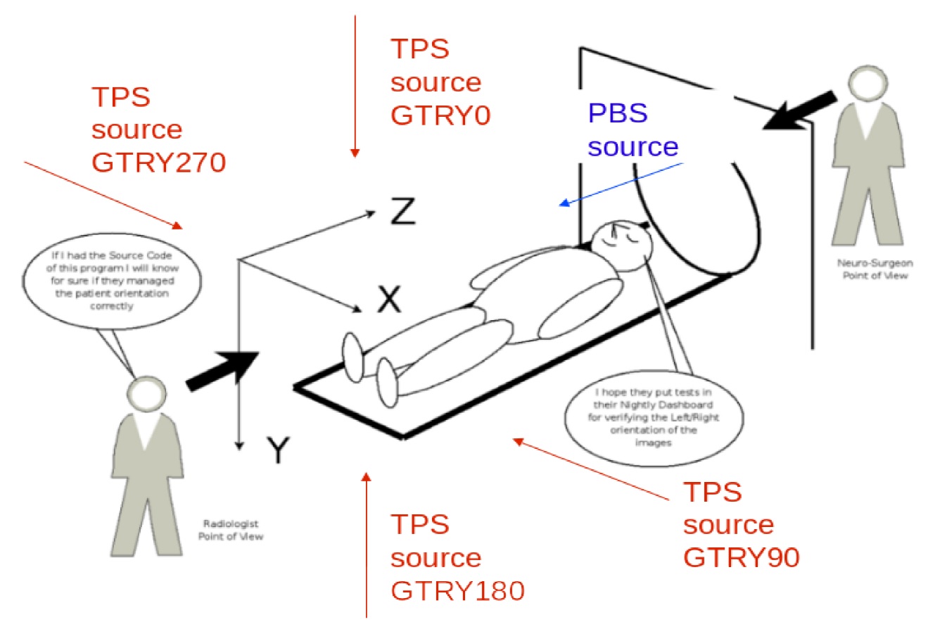
Fig. 6.4 TPS coordinate
The TPS PencilBeam source (TPS) consists in a collection of PencilBeam sources and DICOM image coordinate system is considered as shown in the picture. Relationship between the two sources (from IEC coordinates to DICOM coordinates) is summarized in the table below:
PBS source (+X, +Y, +Z) |
|
|---|---|
Gantry 0 |
TPS source (+X, +Z, +Y) |
Gantry 90 |
TPS source (+Y, +Z, -X) |
Gantry 180 |
TPS source (-X, +Z, -Y) |
Gantry 270 |
TPS source (-Y, +Z, +X) |
Activated default options: SUMMARY
TPS source characteristic |
Active option by default |
Related command |
|---|---|---|
Spot weight (intensity) |
Number of Monitor Unit (MU) |
setSpotIntensityAsNbIons false |
Dose scoring weight |
Set to 1 |
setFlatGenerationFlag false |
Spot delivery |
Random (stochastic fashion) |
setSortedSpotGenerationFlag false |
Beam convergence |
Divergent |
setBeamConvergence false |
Beam energy spread* |
Percentage |
setSigmaEnergyInMeVFlag false |
*warning: it can be overwritten based on your source description file!
6.4. The fastY90 source
The fastY90 source will be part of GATE release 8.0, but it is also available in the development versions of GATE 7.2 availiable on GitHub as of June 2016
The fastY90 source can be used to simulate PET or SPECT imaging of Y90 sources. Rather than simulating the full electron transport of the emitted beta particle, the fastY90 source uses a pre-calculated bremsstrahlung kernel to generate the photons directly to speed up the simulation. Note that since the kernel has been calculated using a point source in water, simulations that use this source are only valid for modelling sources inside water or materials of similar density and Zeff. For accurate simulation, the attenuating media must also extend somewhat beyond the range of the source by several mm. Although the size of the pre-calculated kernel has a radius of 12 mm, more than 95% of all bremsstrahlung is generated within 6 mm of the source, a higher fraction if only the higher energy bremsstrahlung is considered.
The fastY90 model includes the positron arising from internal pair production (0+/0+ transition), though not the 2.186 MeV gamma (2+/0+ transition).
To use the fastY90 source:
/gate/source/addSource mySource fastY90
Simuations with the fastY90 source can be further sped up by adding a low energy cutoff to the bremsstrahlung generation, effictively ignoring those bremsstrahlung photons with too little energy to play any role in imaging. For example:
/gate/source/mySource/setMinBremEnergy 50 keV
The Y90 decay produces a positron with a prevalence of about 31.86 ppm. Although the model defaults to this value, it can be modified (for testing purposes, for example) by the setPositronProbabiliity command:
/gate/source/mySource/setPositronProbability 0.00003186
Using a voxelized distribution with the fastY90 source
The fastY90 source can be used with a voxelized distribution. The voxelized distribution must be in the Interfile format, with a header file that contains, at minimum, the name of the data file, the matrix size, and the scale factor:
/gate/source/mySource/loadVoxelizedPhantom tia_map.h.hdr

!INTERFILE :=
!name of data file :=tia_map.v
matrix size[1] := 256
matrix size[2] := 256
matrix size[3] := 147
scale factor (mm/pixel) [1]:= 1.91
scale factor (mm/pixel) [2]:= -1.91
scale factor (mm/pixel) [3]:= -2.00
The data file must be a raw binary containing data in IEEE 32-bit floating point format. The voxelized distribution will be scaled internally to create a 3D probability map of the geometry of the source, but the total activity is set by the setActivity command as for any other source. By default, the location of the voxelized source will be centred at the origin. The position of the voxelized distribution can also be changed using the setVoxelizedPhantomPosition command to specify the position of the first pixel in the data file:
gate/source/mySource/setVoxelizedPhantomPosition -3.5 6.0 -10.0 cm
6.5. ExtendedVSource
The ExtendedVSource is an extension of the basic GATE’s VSource class, which provides the model for the positronium decay.
All properties of VSource source are inherited by ExtendedVSource.
Two positronium decays channels are provided: two-photon decay (parapositronium (pPs) decay) and three-photon decay (orthopositronium (oPs) decay). Additionally, it is possible to add de-excitation (prompt) gamma to the decay model.
6.5.1. Creating a source
To create a source use command:
/gate/source/addSource NAME Extended
and choose the model:
/gate/source/NAME/setType MODEL
There are 4 possible models:
sg - single photon emission
pPs - two-photon emission from pPs decay
oPs - three-photon emission from oPs decay
Ps - mixed emission ( mixed photon emission from oPs and pPs decays )
Additionally one can add a prompt gamma emission (gamma emitted during the de-excitation).
To do that use a command:
/gate/source/NAME/setEnableDeexcitation true
/gate/source/NAME/setPromptGammaEnergy ENERGY UNIT
ENERGY is a float number, UNIT is energy unit (eV, keV, MeV, …)
6.5.2. Other commands
For all models following commands are available:
setFixedEmissionDirection - set fixed emission direction of single gamma or prompt gamma:
/gate/source/NAME/setFixedEmissionDirection X Y Z
setEnableFixedEmissionDirection - set enable/disable fixed emission direction of single gamma or prompt gamma:
/gate/source/NAME/setEnableFixedEmissionDirection true
For sg model there is a dedicated command to set emitted photon energy setEmissionEnergy:
/gate/source/NAME/setEmissionEnergy ENERGY UNIT
The positronium mean lifetime can be set for the following models: pPs, oPs and Ps . The mean lifetime values in the vacuum are used as defaults. The lifetime per event is randomly chosen from the exponential distribution. Each annihilation gamma has time increased by this value. To set the mean positronium lifetime use a command setPostroniumLifetime:
/gate/source/NAME/setPostroniumLifetime POSITRONIUM TIMEVALUE TIMEUNIT
where POSITRONIUM is a name of positronium type (pPs or oPs), TIMEVALUE is float number, TIMEUNIT is time unit (ns, ps, …).
For the Ps model it is required to define a fraction (normalized to 1) of emitting photons from pPs and oPs decay. User must define a fraction for one type of positronium - the second one will be calculated automatically. To do that use a command setPositroniumFraction:
/gate/source/NAME/setPositroniumFraction POSITRONIUM PROBABILITY
where POSITRONIUM is a name of positronium type (pPs or oPs), PROBABILITY is a float number in range from 0 to 1.
6.5.3. Dedicated branches
For this source 4 additional branches are present in the Hits tree:
gammaType - describes the type of the gamma
sourceType - describes the source type
decayType - describes from which decay channel of positronium is emitted gamma
decayIndex - branch present in the output format, but not filled by
ExtendedVSource
Int is the type of value stored in all four branches. Meaning of values in gammaType, sourceType and decayType is described in the tables below.
Value |
Description |
|---|---|
0 |
photon/particle without emitted-gamma metadata |
1 |
single photon (emitted by sg model) |
2 |
annhilation gamma |
3 |
prompt gamma |
Value |
Description |
|---|---|
0 |
photon/particle without emitted-gamma metadata |
1 |
single gamma emitter (sg model) |
2 |
parapositronium (pPs) |
3 |
orthopositronium (oPs) |
4 |
direct annihilation without positronium formation; not emitted by ExtendedVSouce |
Value |
Description |
|---|---|
0 |
unknown decay |
1 |
standard decay channel (pPs–>2 gamma, oPs–>3 gamma) |
2 |
de-excitation and decay channel (pPs–>2 gamma + prompt, oPs–>3 gamma + prompt) |
For ExtendedVSource, the decayIndex branch is not set by the source model and therefore always keeps the default value -1.
6.6. PositroniumSource
The full theoretical description of the model, together with implementation details and tests, is available in A Monte Carlo positronium decay source model with multiple annihilation channels in GATE.
PositroniumSource is a dedicated source model for positronium decays. It combines the standard source activity, time and position handling from GateVSource with an internal decay model that generates:
a delayed 2-gamma or 3-gamma annihilation vertex,
an optional prompt de-excitation gamma,
an optional spatial shift of the annihilation point to model the mean positron range.
The source is configured component-by-component. Each component represents one positronium decay channel description with its own intensity, lifetime and prompt-gamma settings.
6.6.1. Creating a positronium source
Create the source with the dedicated source type and then set its internal model type to Ps:
/gate/source/addSource NAME PositroniumSource
/gate/source/NAME/setType Ps
As for other sources, the activity and the spatial or temporal distributions are configured with the standard source commands, for example:
/gate/source/NAME/setActivity 1000 Bq
/gate/source/NAME/gps/pos/type Point
/gate/source/NAME/gps/centre 0. 0. 0. mm
The annihilation particles are generated internally by the positronium model, therefore there is no need to configure gps/particle, gps/energytype, gps/monoenergy or angular GPS settings for the annihilation gammas.
6.6.2. Component parameters
All positronium-specific commands are available under /gate/source/NAME/.
6.6.2.1. Required commands
/gate/source/NAME/setPositroniumFractions f1 f2 ... fnRelative weights of the configured components. The implementation normalizes the vector internally, but the values should represent the intended relative intensities.
/gate/source/NAME/setPositroniumLifetimes t1 t2 ... tn unitLifetime of each component. The last token is a Geant4 time unit such as
ns./gate/source/NAME/setPromptPhotonProbabilites p1 p2 ... pnProbability of prompt-gamma emission for each component. Values are restricted to the
[0, 1]range by the messenger./gate/source/NAME/setPromptPhotonEnergies e1 e2 ... en unitPrompt-gamma energies for each component. The last token is a Geant4 energy unit such as
keVorMeV.
One of the following commands must also be provided:
/gate/source/NAME/setDecayKinds k1 k2 ... knExplicit annihilation channel selection for each component. Allowed values are
k2Gammaandk3Gamma./gate/source/NAME/setPositronInteractions k1 k2 ... knInteraction type assigned to each component. Allowed values are
kParaPs,kDirectandkOrthoPs. This command is used by the model to derive thesourceTypemetadata stored in the Hits tree. It can also be used instead ofsetDecayKindsto derive the 2-gamma and 3-gamma contributions from the theory.
Note
The current implementation can build the decay model from setDecayKinds alone, but the sourceType metadata in the Hits tree is derived from setPositronInteractions. In practice, if you want a fully consistent PositroniumSource configuration and meaningful sourceType values, define setPositronInteractions as well.
6.6.2.2. Optional commands
/gate/source/NAME/setElectronCaptureProbabilities p1 p2 ... pnProbability that the positron is lost by electron capture and no annihilation vertex is produced for a given component. If this command is omitted, all probabilities default to
0. Values are restricted to the[0, 1]range./gate/source/NAME/setMeanPositronRange r1 r2 ... rn unitMean positron range for each component. When this command is set, the annihilation vertex is shifted with an isotropic 3D Gaussian whose mean displacement matches the supplied range.
Note
In the explicit setDecayKinds workflow, all parameter vectors must describe the same number of components. This applies to the fractions, lifetimes, decay kinds, prompt-gamma probabilities, prompt-gamma energies and, when used, electron-capture probabilities and mean positron ranges.
Note
The current implementation requires both setPromptPhotonProbabilites and setPromptPhotonEnergies even when the prompt-gamma probability is zero for all components. A common convention is to set the corresponding energies to 0.
6.6.3. Event timing and generated vertices
For each event, the source first samples the source time and position from the standard source configuration. Then the positronium model may generate up to two primary vertices:
a prompt-gamma vertex at the sampled source time and position,
an annihilation vertex delayed by an exponential law with the configured positronium lifetime.
If setMeanPositronRange is used, the annihilation vertex position is additionally smeared around the sampled source position.
If the electron-capture probability is very high and the prompt-gamma probability is very low, event generation can become inefficient because the source retries until at least one primary vertex is created. The code emits a warning when the probability of producing neither a prompt gamma nor an annihilation exceeds 90% for a component.
6.6.4. Dedicated Hits branches
Hits produced by PositroniumSource carry four additional integer branches in the Hits tree:
gammaType - type of emitted gamma,
sourceType - physical origin of the gamma,
decayType - decay model attached to the sampled component,
decayIndex - zero-based index of the sampled decay component.
The decayIndex value is copied to all gammas emitted from the same sampled component. In the explicit setDecayKinds workflow, the index follows the order of components in the user-defined vectors. When the source is configured through setPositronInteractions, the helper may internally expand one user component into several annihilation channels, so decayIndex refers to the final internal component list used by the model.
Value |
Description |
|---|---|
0 |
photon/particle without emitted-gamma metadata |
1 |
single photon from the |
2 |
annihilation gamma emitted after positronium decay |
3 |
prompt gamma emitted in the de-excitation part of the decay |
Value |
Description |
|---|---|
0 |
photon/particle without emitted-gamma metadata |
1 |
single gamma emitter; not emitted by |
2 |
parapositronium component (pPs, 2-gamma annihilation) |
3 |
orthopositronium component (oPs, 3-gamma annihilation) |
4 |
direct annihilation without positronium formation |
The values observed in sourceType are assigned by GatePositroniumDecayModel::GetSourceKind from the sampled interaction kind. For this reason, meaningful sourceType values require setPositronInteractions to be configured.
Value |
Description |
|---|---|
0 |
decay model not defined for this particle or metadata unavailable |
1 |
standard decay channel (annihilation only) |
2 |
de-excitation and decay channel (prompt gamma plus annihilation) |
Value |
Description |
|---|---|
-1 |
decay index not defined for this particle or metadata unavailable |
0, 1, … |
zero-based index of the sampled decay component stored in the model |
6.6.5. Minimal example
The example below defines a two-component source with explicit 2-gamma and 3-gamma channels, a prompt gamma accompanying both components and a finite mean positron range:
/gate/source/addSource psSource PositroniumSource
/gate/source/psSource/setType Ps
/gate/source/psSource/setActivity 1000 Bq
/gate/source/psSource/gps/pos/type Point
/gate/source/psSource/gps/centre 0. 0. 0. mm

/gate/source/psSource/setPositroniumFractions 0.25 0.75
/gate/source/psSource/setPositroniumLifetimes 0.125 142.0 ns
/gate/source/psSource/setDecayKinds k2Gamma k3Gamma
/gate/source/psSource/setPositronInteractions kParaPs kOrthoPs
/gate/source/psSource/setPromptPhotonProbabilites 1.0 1.0
/gate/source/psSource/setPromptPhotonEnergies 1.274 1.274 MeV
/gate/source/psSource/setElectronCaptureProbabilities 0.0 0.0
/gate/source/psSource/setMeanPositronRange 0.2 0.2 mm
In this setup, each sampled decay produces a prompt gamma at the source position and a delayed positronium annihilation. The first component annihilates into 2 gammas, while the second one annihilates into 3 gammas.